Introducing Matrices
|
Matrices (not to be confused with mattresses, those springy things that we lie on bed!) are mathematical constructs which can be used in a number of ways such as the solution of simultaneous equations (which you have probably already seen. If you've been to that section already) but their origin if you like lies in network diagrams such as for dataflow and possibly water flow in a network of water pipes. |
|

Take for example the following simple diagram which could be used to model data flow, or as I said before water flow in a network of water pipes.
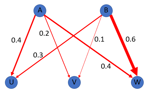
You may be able to see already that the rate at which water for example will flow along the pipe would depend on the width of the pipe. A small 22 mm water pipe in your house would not be able to handle the flow rate of the large 1 m (or above) diameter mains pipe that runs down your main road. Of course, if this was a network data model the capacities of the "pipes" (cables) would not be quite so obvious, data cables are not necessarily thicker (generally, although there are quite thick ones running along the seabed) so this model is deliberately visual.
You can see that if a fixed amount of data (water) entered at Node A, the amounts of water reaching Nodes U and V would differ due to the different capacities of the connecting pipes (cables).
Q1. Consider the diagram. How much water is output at Nodes U, V and W if the only inputs is 1 L of water at Node B?
A1. You should be able to see from the data capacity of each type (cable) that proportionally 0.3 fraction of 1 L would arrive at node U, 0.1 fraction of the litre would arrive at node V and 0.6 fraction would arrive at node W. Therefore the volumes would be 300 mL, 100 mL and 600 mL respectively.
Q2. How much water is output at the nodes U, V and W if the only input of water is 2 L at node A?
A2. Again you should be able to see that the water deposited at node U would be 800 mL (0.4×2), the water deposited at node V would be 400 mL (0.2×2) and the remainder arriving at node W would be also 800 mL (0.4×2) as pipelines AU and AW have the same capacity.
You can of course invert the calculation and calculate the quantities of data/water released from a particular point given the arrival quantities and capacities of the pipes.
If, this time we take a look at a slightly modified version of the above diagram we can model this. We can then take another step forward and utilise variables as opposed to fixed quantities and while this may seem to complicate issues it does in fact make the whole idea of this sort of model more useful.
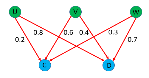
Q3. How much water would be output at nodes C and D if 1 L of water is input at Node U and 2 L of water at Node V. There is no water input at Node W.
A3. Again we use the given pipe capacities as multipliers. Consider the input at Node U. 1 L of water input here will give 200 mL at Node C and 800 mL at Node D. Similarly 2 L of water input at Node V will give 1200 mL of water at no C and 800 mL of water at Node D
The totals therefore would be:
Node C equals 200+1200 = 1400 mL
Node D equals 800+800 equal 1600 mL
Now then, you should know by now that mathematicians don't like things to be this straightforward, to preserve their mysterious status they like to confuse and obfuscate by substituting algebraic variables where numbers would normally live. Let's take a look at a problem using algebraic variables.
Q4. How much water would be output at Nodes C and D if 'x' litres of water were input Node U, 'y' litres of water were input at Node V and 'z' litres of water were input at Node W?
A4. If you study the diagram, paying attention to the inputs at each node and the capacities given for each pipeline (cable) you should be able to work out the following:
Node C = 0.2x +0.6y +0.3z
Node D = 0.8x +0.4y +0.7z
Hopefully you can see that the totals for x, y and z respectively all come to 1.
Now then, before we leave this section will take a look at what we can do if we combine both networks. This can get quite confusing so if you haven't already given up by now :-) take it slowly.
Take a look at the diagram that shows both of the previous networks joined together so that inputs from A and B will ultimately feed C and D by passing through one or more nodes UV or W.
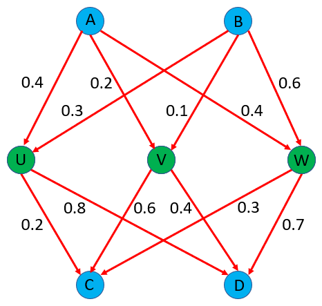
Q5. Calculate the amount of water arriving at Node D if the only input is 1 L of water at Node A.
A5. It is important that you trace the path carefully and consider using the capacities given as decimal multipliers.
Step 1 - 1 L of water entering the system at node A would deliver 400 mL at node U, 200 mL of water at node V and 400 mL of water at node W.
Step 2 - node U will deliver 0.8×400 mL to node D, node V will deliver 0.4×200 mL to node D and finally node W will deliver 0.7×400 mL to node D. Stop at this point and study the diagram and the figures until you are happy that you can see why these values are correct and how they were obtained.
Now we need to carry out the multiplications and add up the totals.
Node D will receive : (0.8 x 400) +(0.4 x 200)+(0.7 x 400) = 320mL + 80mL + 280 mL = 680mL of the input 1000mL (0.68L of 1litre).
Q6. Calculate the amount of water arriving at Nodes C and D if the only input is 1 L of water at Node B.
A6. All you have to do is follow the diagram and consider the multipliers as you did for question 5.
Step 1 - the amount of water arriving at node U is 300 mL (0.3×1 L). Similarly the amount of water arriving at node V is 100 mL (0.1×1 L). Finally the amount of water arriving at node W is 600 mL (0.6×1 L) and as you can see these total 1 L, confirming no loss at this stage.
Step 2 - node U provides 0.8×300 mL equals 240 mL to node D. Node B provides 0.4×100 mL equals 40 mL to node D and finally node W provides 0.7×600 mL equals 420 mL to node D. If you add up the volumes you will see that the input at node B provided 240+40+420 = 700 mL, the remaining 300 mL will have gone to node C.
Now that we have introduced some potential real-life applications for matrix algebra, will take a look at what the matrix actually looks like and what we can do with it mathematically.
Back To >> Simultaneous Equations - Solving with Matrices <<