[A] Definite Integrals
Previously we have performed “integrations” or have sought our “antiderivatives” and left them as expressions, without any “definite” value. In much the same way that we might expect an expression like the one below:
To actually yield a result, for example giving ‘x’ a value of 4 would make the above expression return a value for ‘y’:
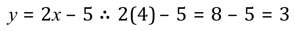
In these cases we would regard the result for ‘y’ as being a definite value.
To make our anti-derivative return a definite value we make the integration itself definite by performing it between upper and lower bounds known as “limits of integration”
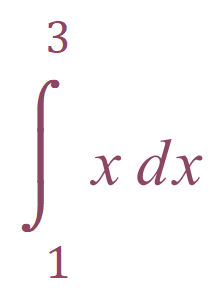
Consider this expression:
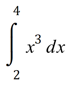
This expression asks you to integrate the value for ‘x’ and having done so substitute the values of the upper and lower bounds to arrive at a final result.

Ironically it is possible to perform the integration correctly but then to get the answer wrong through incorrect substitution of the limits. It pays to take great care when doing this.
Perhaps the main reason, or main use, for “definite integration” would be to evaluate the areas under curves between preset bounds (or limits). Perhaps the simplest curve would be the simple plot of the function y = x:
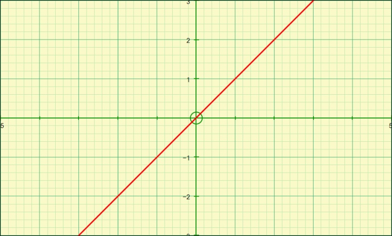
As you can see from the graph above the function gives a straight-line passing through the origin, every point on the curve (although it’s a straight-line we still refer to it as a curve). The diagram below is an annotated version of this curve representing a section of the area underneath it between limits three and one:
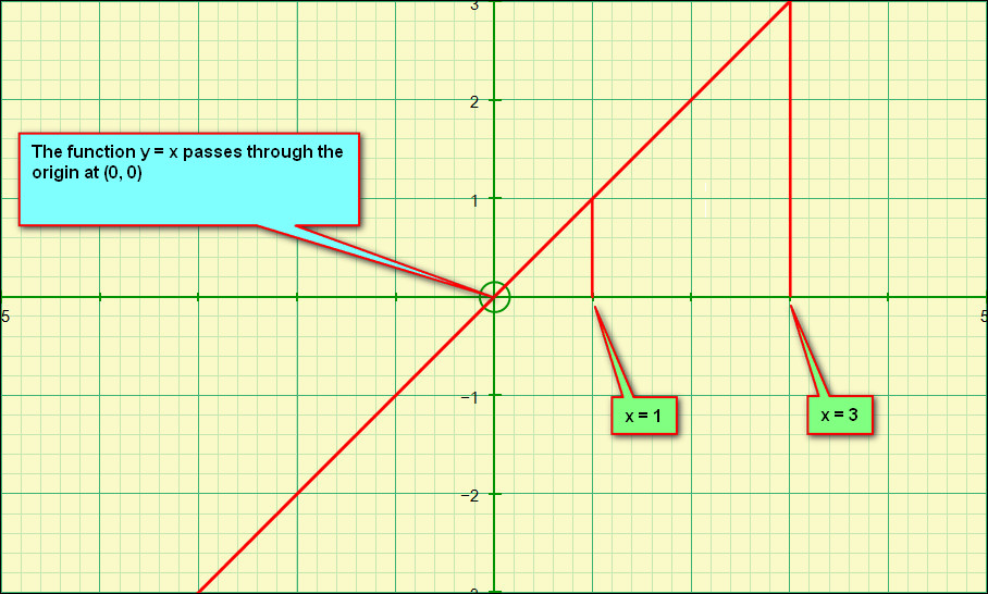
Taking into account the large squares (which comprise each of 25 of these smaller squares) you can quite easily work out the area underneath the “curve” as being exactly 4 units (we can count three whole ones and two halves) but how can we prove this using integration?
The limits of our integral are shown as three and one respectively:
Our function as you can see from the expression above is ready to be integrated between those limits. Let us now perform that integration and prove the above.
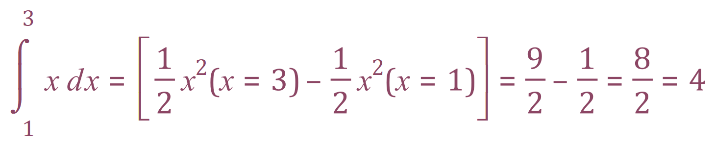
Okay, that wasn’t so bad was it?
Let’s do the same calculation again, but this time we will use the small squares not the large ones. The limits this time then will be 15 and 5 (if you can’t see this, study the graph and look at the small units).
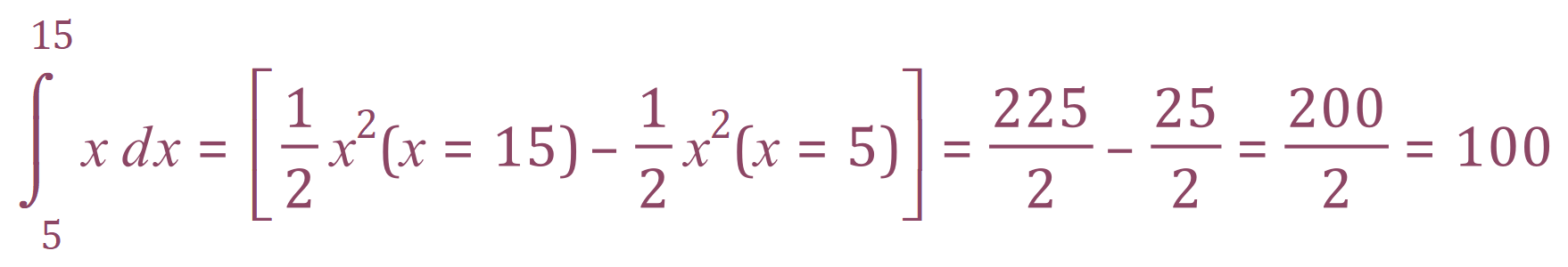
Take a look at the graph and you will see that we have 3 squares made up of 25 smaller ones making 75 small squares and then two “half squares” making up a further 25 which totals 100.
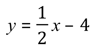
Let’s try a slightly different graph:
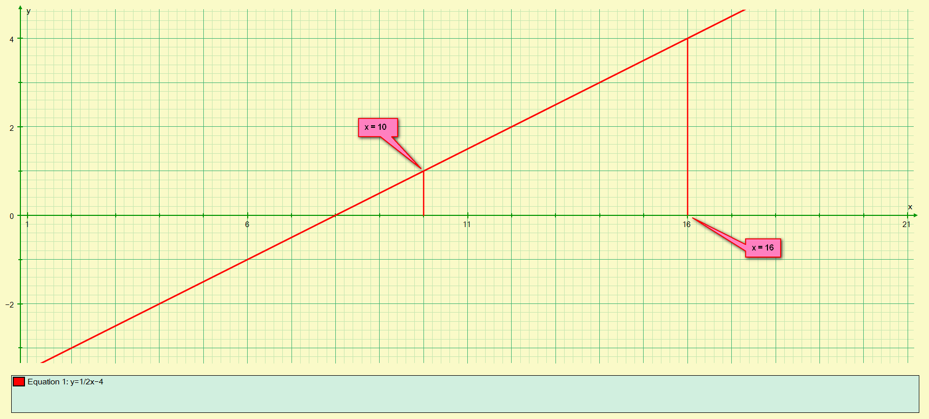
A little bit of careful counting will tell you that between the limits of 16 and 10 we have the effective equivalent of 15 large squares so the result of our definite integral should be 15. Let us now actually make the integration and see if we are correct:
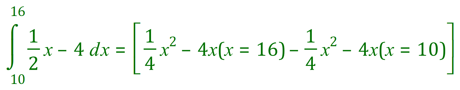
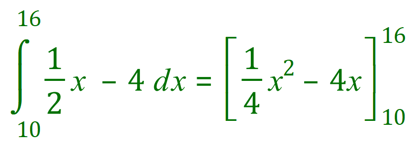

A little bit convoluted I’m sure that you agree but this is the second time now that we have proved our case (count the squares to prove it to yourself).
As I mentioned previously, although the graphs that we have drawn have in fact been straight lines they are still regarded mathematically as “curves”. Where this method comes into its own is when you are actually dealing with curves that are in fact curved (!).
The simplest curve I can think of that is in fact curved would be the plot of:
From the graph below, you can see that this function plots to a parabolic curve passing through the origin at its lowest point, i.e. when x and y both equal zero.
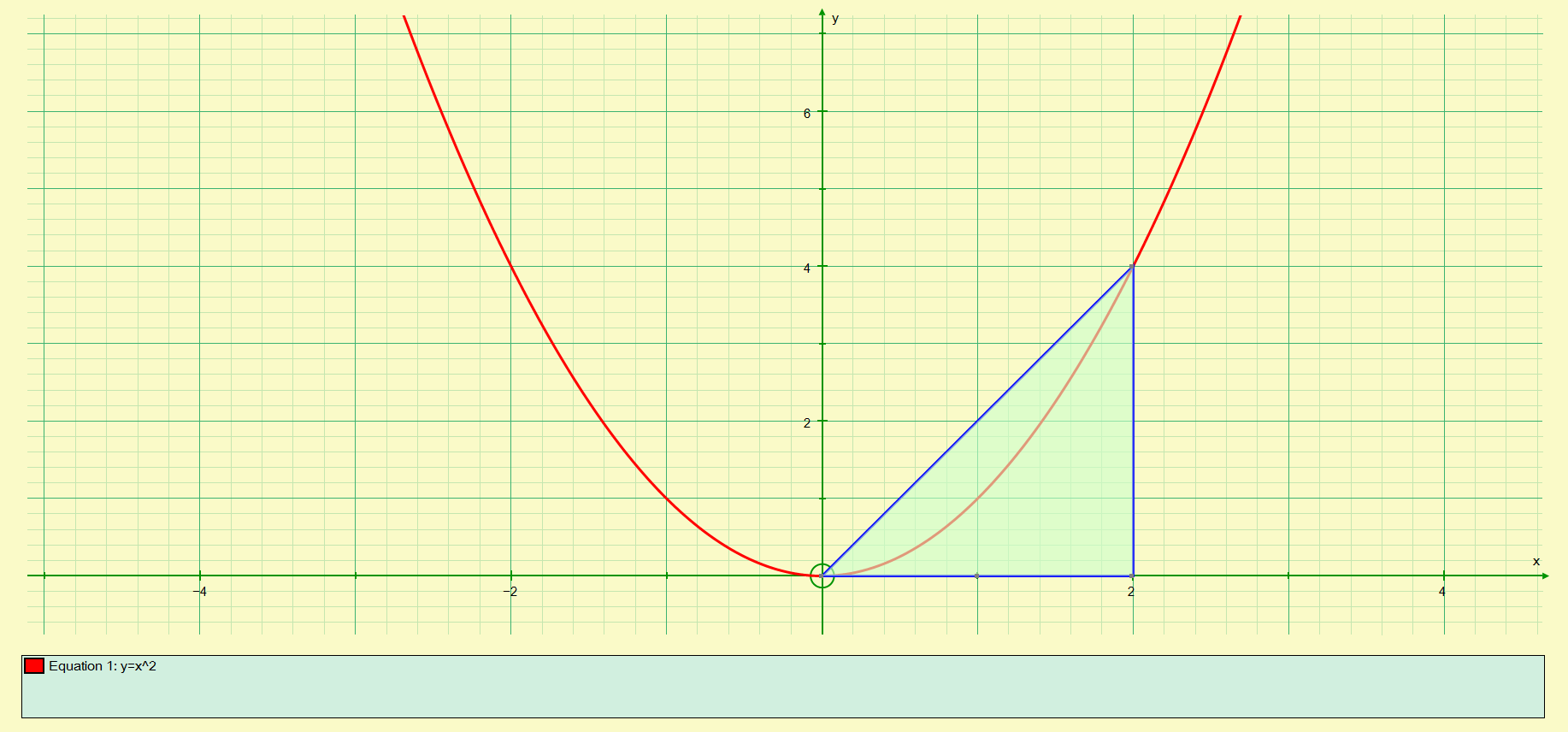
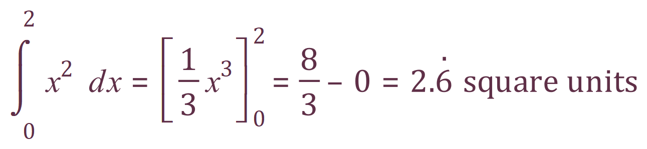
The area under the curve between the limits of 2 and 0 is shown in green, however we have also included a segment above the curve, which we are not interested in. The right angled triangle above has an area of 4 square units (remember 1/2 b x h).
But we only want the area under the curve. Now this time it’s not so easy to count squares because we can’t be exact as to where the curve cuts through any particular square, so we have to rely on integration.
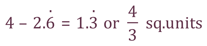
A particularly demanding maths examiner might ask you for the area of the section above the curve, in this case it would be:
This method for finding the area under curves comes into its own when we start looking at more complicated functions.
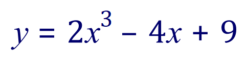
Let us look at a more complicated function:
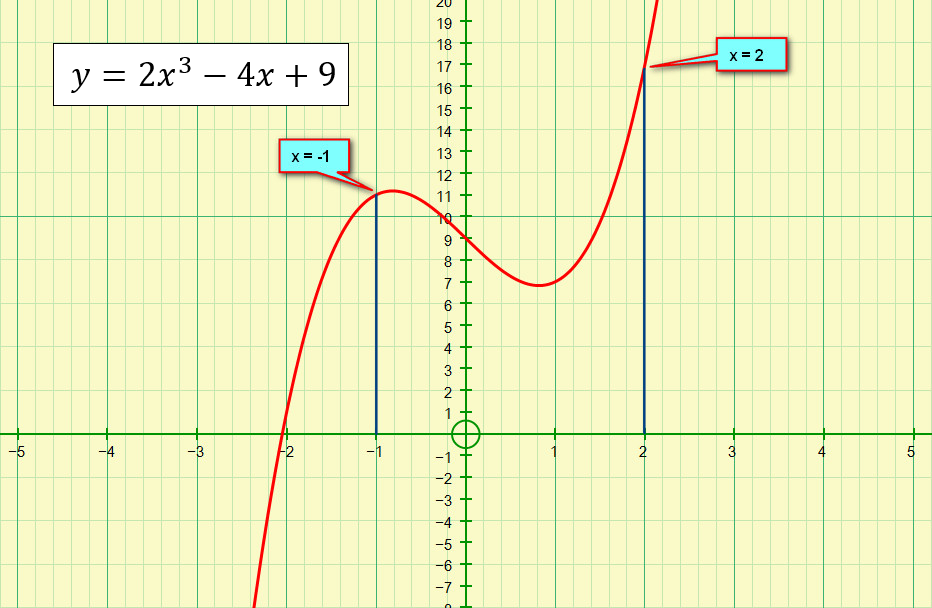
The two vertical blue lines at x = 2 and x = -1 are the limits of the integration that we wish to perform. The area that we are interested in underneath the curve lies between these limits and the contour of the curve of the function.
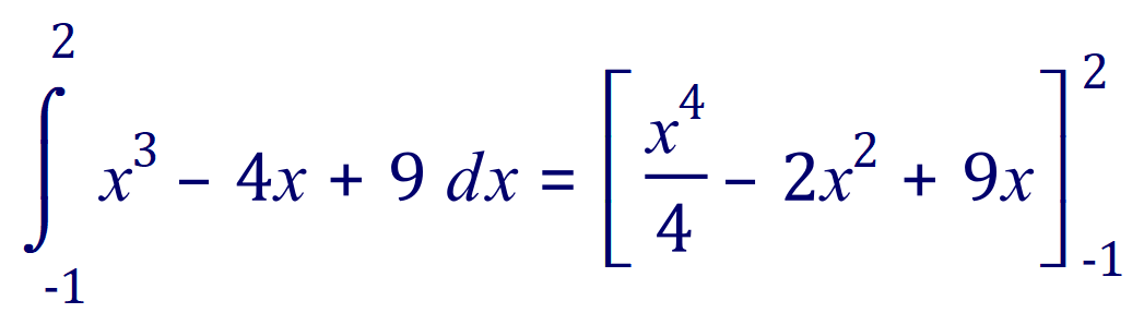
Let us integrate this function and evaluate the value in square units of the area bounded.

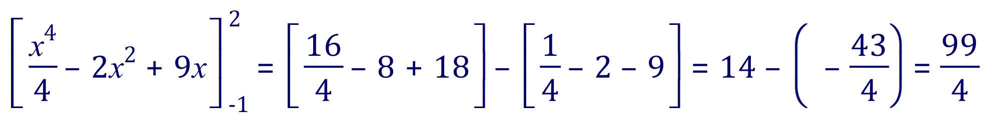
Or 24.75 square units.
If you look at the curve above you will see that between the limits -1 and +2 a certain part of the curve is traced out, if you can imagine that rotated through 360° along the x-axis you will end up with a three-dimensional solid which would look very much like a solid version of a very ornate vase or fruit bowl. These “Three-Dimensional Tracings” are called “Volumes of Solids of Revolution” and looking at these will be the next feature of this particular part of our journey through calculus.