Differentiation
It is fair to say, each branch of mathematics has its uses, distinctions and defining points. When we consider geometry we are looking at shapes and the relationships between them and when we look at algebra we are looking at variables and their uses in solving equations.
Calculus is the branch of mathematics that deals with change and it falls into two branches:
- Differential calculus, which deals with the rate of change and slope of curves.
- Integral calculus, which deals with the accumulation of quantities and the areas underneath and between curves.
It is logical to deal with differential calculus before we explore integral calculus, and to quote a famous line from a film “Stand and Deliver” (starring Edward J Olmos and Lou Diamond Phillips) “calculus was not designed to be easy, it already is”. An excellent film, but I don’t fully agree with that statement because calculus can be complicated and there are many rules which must be learned and strictly applied if you’re going to get anywhere in this fairly deep and complicated branch of mathematics.
When we look at differential calculus, we are observing the rate of change of a function, plotted as a curve.
Let us consider the simple function:
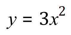
We can see that:
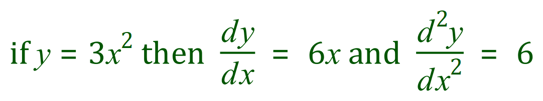
What we need to establish is how?
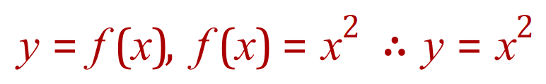
The example I have used above, is probably not the best one (as it involves a constant multiple, a rule which we will visit later) certainly not to display the “first principles” rule of differentiation. I’m going to drop back to a simpler function:
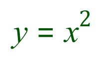
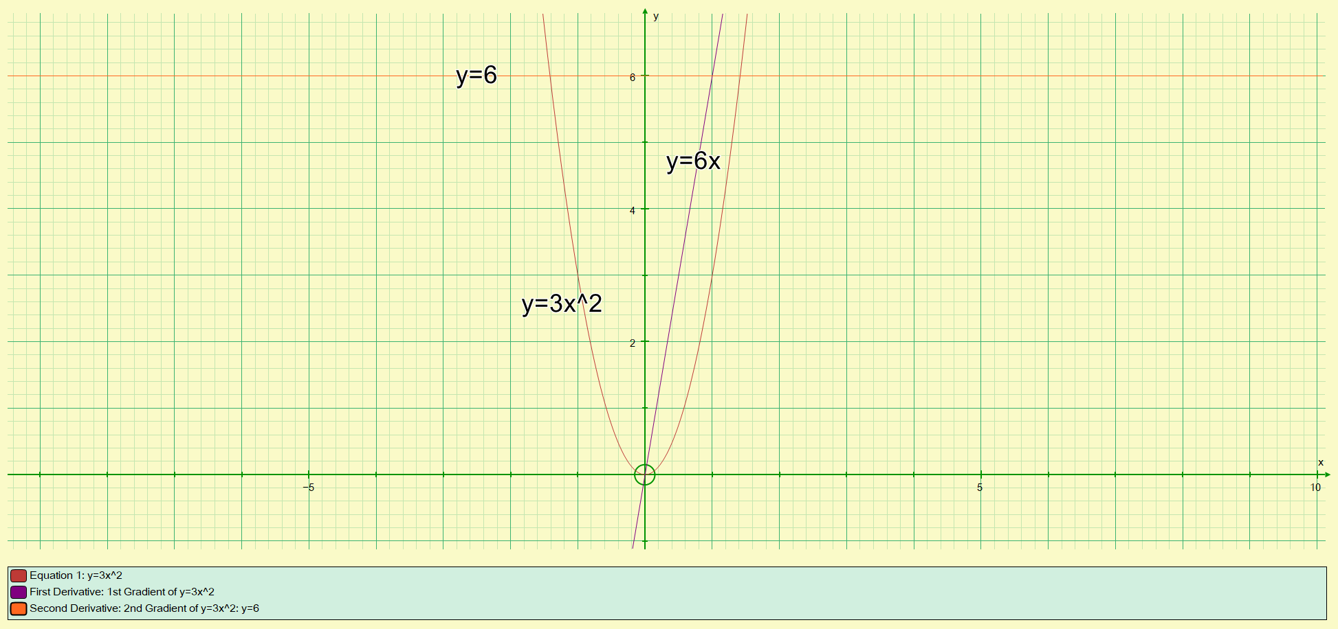
Perhaps the simplest curve you’ll come across, but it gives a similar curve to the one above. Look at the picture below, you can see the plot of the function in just the same way as the one above:
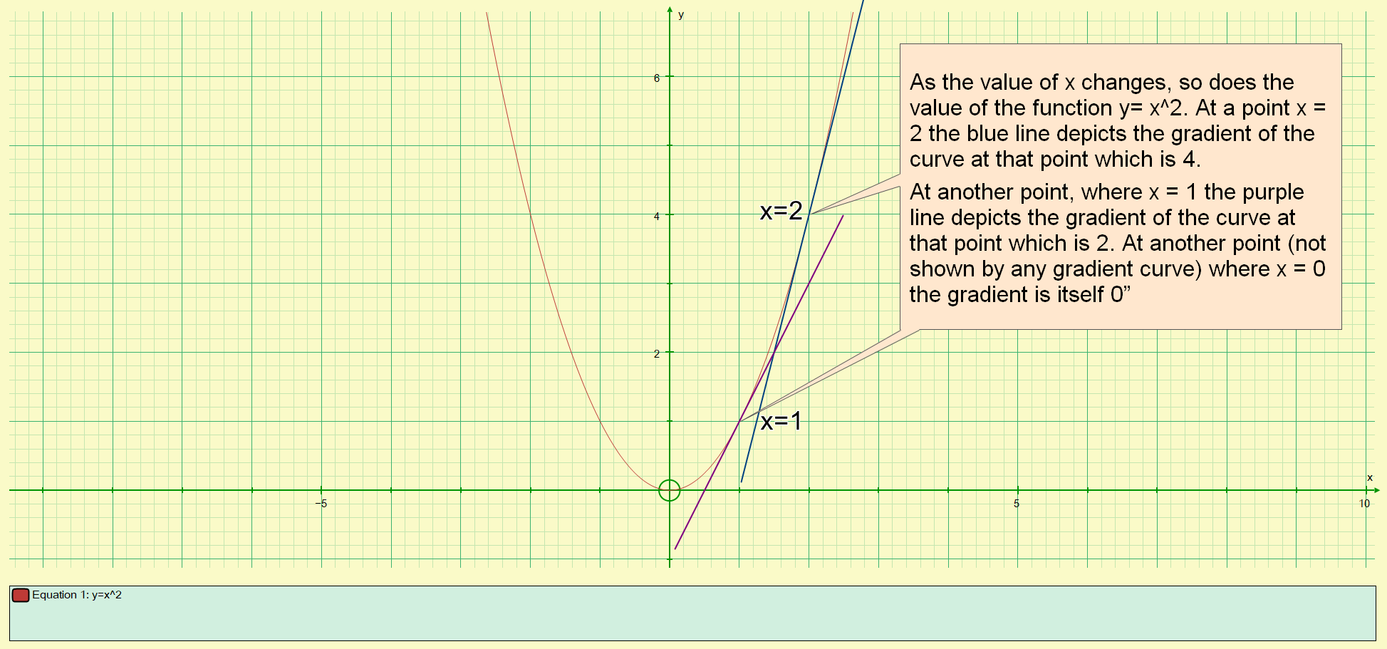
Once again, you can see that the values of the gradient at each given value of X satisfies our previous conclusion that is the first and second derivatives but was still haven’t shown how we get there.
Now I think it is time to go through the mechanics of how we arrive at the generic expression for a first derivative.
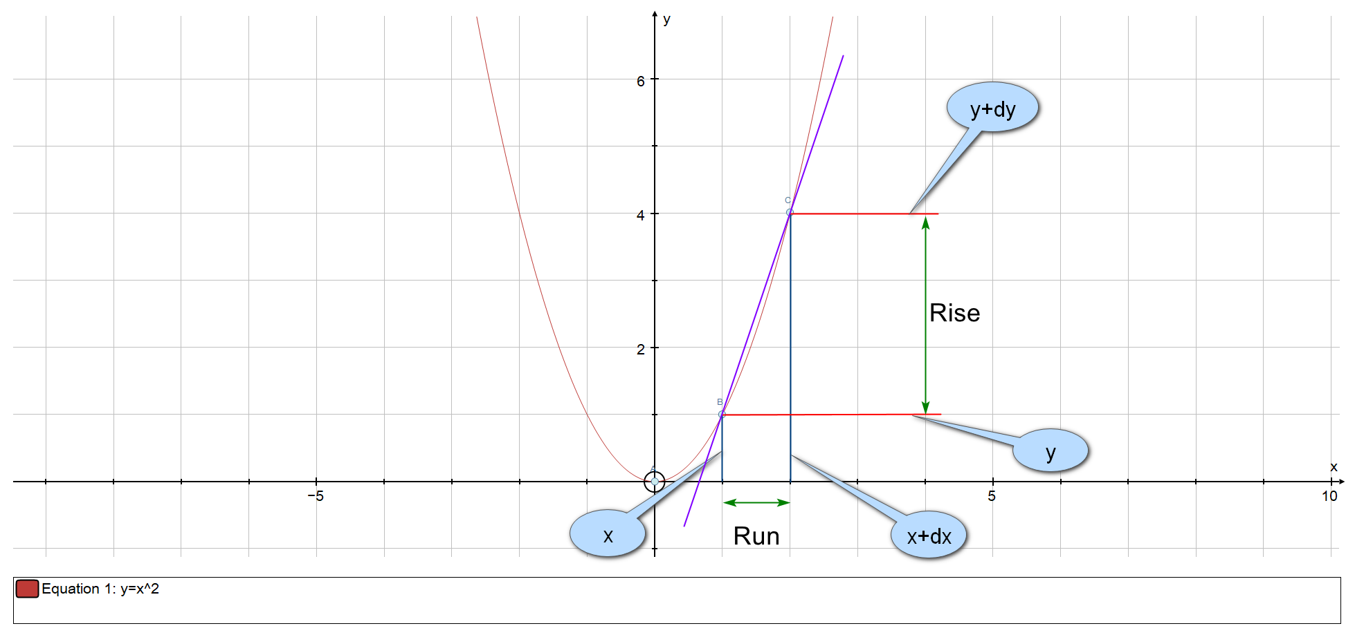
Consider the plot of the function:
The lowest point on the curve shows the value of ‘y’ for the particular value of ‘x’. When there is a change in ‘x’ there is a commensurate change in the value of the function ‘y’ and this is shown by the second point on the graph. The change between ‘x’ and the ‘x plus a little bit’ is labelled “run” and the change in ‘y’ between ‘y’ and ‘y plus a little bit’ is labelled “rise”.
Generally in science, the ‘little bits’ are denoted using the Greek letter Delta (or occasionally, the lower case 'd' (in certain branches of chemistry and physics this is shown as a small triangle but in mathematics we use the actual letter Delta.
Let us now return to our function:
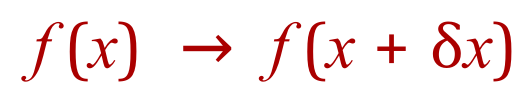
If there is a small change in our function so that:
Then there will be corresponding change in ‘y’:
If we compare the change in ‘y’ to this change in ‘x’ then we write this by putting into symbols the expression “the change in ‘y’ with respect to ‘x’:
What you are in fact looking at is the gradient between the two points, otherwise known as the “rise” divided by the “run”. The change in ‘y’ is represented symbolically as we have seen as  .
.
Take a good look at the expression below:
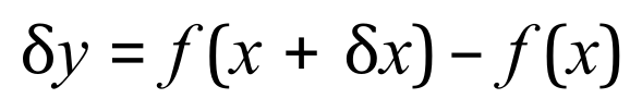
What this is actually saying (and if you study this in conjunction with the picture on the previous page) is that the change in ‘y’ is actually the difference between the new value of f(x) and the old value. If we compare this with the change in ‘x’ we arrive at this expression:
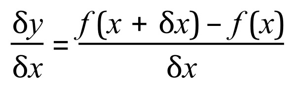
Now if we consider that our function is y = x^2 we can substitute this into the above expression and we arrive at the following:
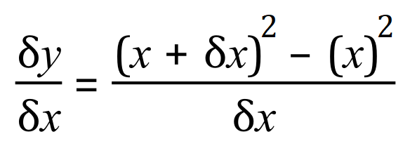
If we expand, we get this:
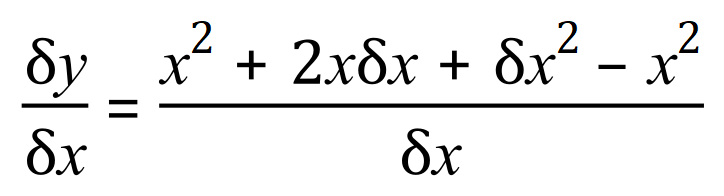
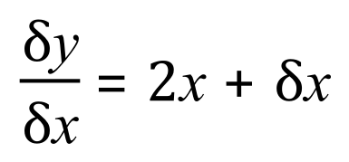
We can see that the ‘x’ squared terms on the right hand side disappear and if we cancel on the right-hand side by 'Delta x' we are left with:
As the change in ‘x’ reduces to its limit of zero (the value of ‘delta x’ tends to 0) therefore the change in ‘y’ with respect to ‘x’ as we zero in on that specific point on the graph becomes 2x.
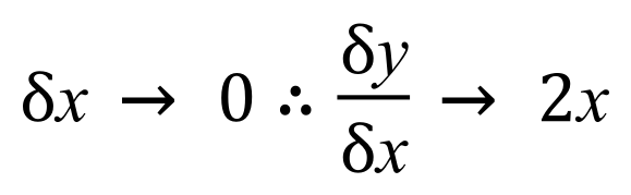
Therefore we can say:
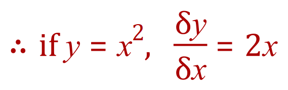
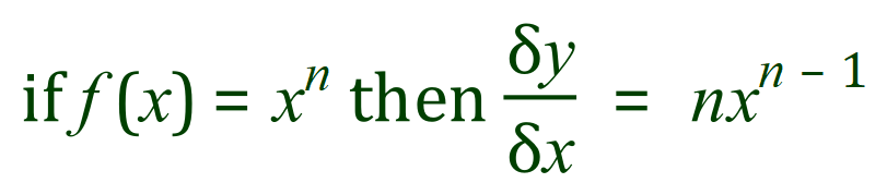
In other words the first derivative of the function y=x^2 is 2x. This leads us naturally to the first ‘generalisation’ in differentiation:
>> Questions <<
>> Table Of Standard Derivatives And Integrals <<
Back To >> Tangent To A Curve <<