Mean Mode and Median
In this section we will start to talk about "mean", "mode" and "median". If we were to take the weights of, so for example a class of 30 students, we may be interested to know the weight of the lightest student, the weight of the heaviest student and an average weight across the whole class. "Average" is another word for "Mean" and is obtained by adding up the total of (in our case weights) the numbers in the dataset, and then dividing the total by the number of items in the dataset.
A short example might clarify this:
Consider the numbers: 25, 30, 35 and 40. Straight away we can see that we have 4 items in the dataset, and if we add them all up we arrive at the value of 130. If we then divide 130 by 4 we arrive at the average or mean value of 32.5.
Another example might be the average fuel economy of a car over a six-month period:
Jan = MPL (8.4), Feb = MPL (7.9), Mar = MPL (8.1), Apr = MPL (9.7) May = MPL (8.2) and Jun = MPL (8.0)
Considering the first 6 months of the year, the MPL (miles per litre) values can be "averaged" and the "mean" value arrived at. Statistics are useful and can often tell us a lot about the subject they represent, for example why do you think that the MPL in April is so much higher than in any of the other months? Well, It could be that during that month, the driver took a lot of journeys on the motorway, long straight journeys with fewer starts and stops can do quite a bit to improve the economy of a car.
We now know what the "Mean" is, let's take a look at another dataset where we can identify the remaining two statements.

The data above shows the individual shoe sizes of 19 students in a class. If we add up the values of all 19 students and divide by 19 we come to a "Mean" of 153 with an average shoe size of size 8. We might be interested in some of the features of this dataset, for example the largest size which we can see is 12, the smallest size which we can see is 5 but sometimes more interestingly the value that seems to be the most common or the value that is in the middle of the dataset. In the first case the most common value is known as the Mode or Modal value, and in the second case the middle value (when the data has been put in order from smallest to largest) which is known as the Median value.
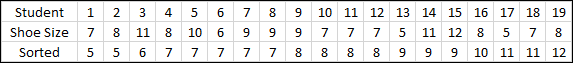
Even a simple job like sorting the shoe sizes into numerical order makes the data a little bit easier to interpret. We can see straight away that the smallest size is 5 and that the largest size is 12, we now have a range of values which means our seemingly random data is now starting to become useful information. We said previously that the median size would be the middle value. We have 19 values so the middle value is going to be the one lying in position 10. We can see that this is actually 8, so the median value (the middle value) is size 8. In such a small table it's not difficult to identify the median, but if the table contain hundreds of data items you would hopefully be looking for an easy way to work out the median.
Luckily for us, there is a way:

If we take the total number of items (in this case 19) as a value for "n", we can see that the median value will lie at position 10 as I said previously. A slight complication can arise when we have an even number of data items. In the previous example we have 19 data items, so the will be a "middle value" if we write the numbers down (this will be the value lying at position number 10). What do we do though, if we have an even number of data items? There isn't actually a "middle value" so we take the two values lying either side of where the middle would have been, and we take the mean (average) of these two values. This becomes our Median value.
The Mode, or Modal Value is the value which occurs the most often and in classroom situations you will probably do this by inspecting your data. Software such as Microsoft Excel will have functions built into it allowing you to establish these values at the click of a mouse, but when you're learning about this topic I'm afraid that you have to "do the miles".
>> Questions <<