Using Graphs
We have just seen the first method by which to solve simultaneous equations. Subsequently you will see how to solve them by using matrices, which although it is not the simplest method does have an unusual appeal and elegance. The next method we are going to consider is the solution of simultaneous equations using straight-line plots.
If you've not already read the section on graphs of a straight line using the familiar equation y = mx + c you can click >> here << to refresh your memory, of course don't forget to come back!
Let us consider this simple pair of simultaneous equations:
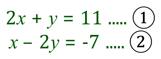
Moving away from the usual method of elimination of one or the other variable and then back substitution of a newly found value for the remaining variable, we can choose to plot these equations as straight-line graphs and identify the solution to the problem by looking at a common point where values for 'x' and 'y' satisfy both equations.... er..... simultaneously 8-).
In order to construct our table of 'x' and 'y' values we now convert, or should I say rearrange, each equation in terms of 'y' and then establish values for 'y' from a suitably chosen range of 'x' values. The table below shows the conversion and appropriate values.
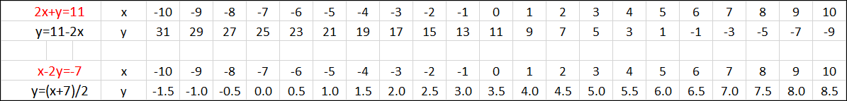
The equation in red shows the unconverted (original) equation and the equation below in black is the transposed equation in terms of 'y'. When we plot the values we have obtained from the calculations, we obtain the following:
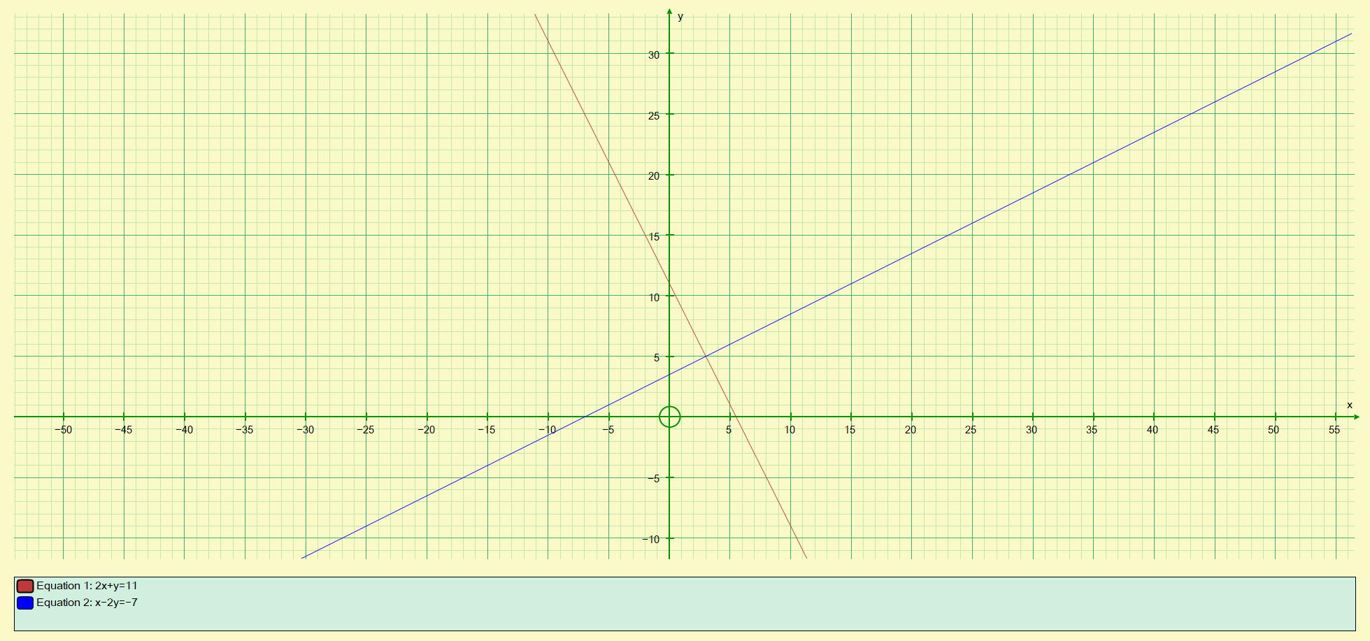
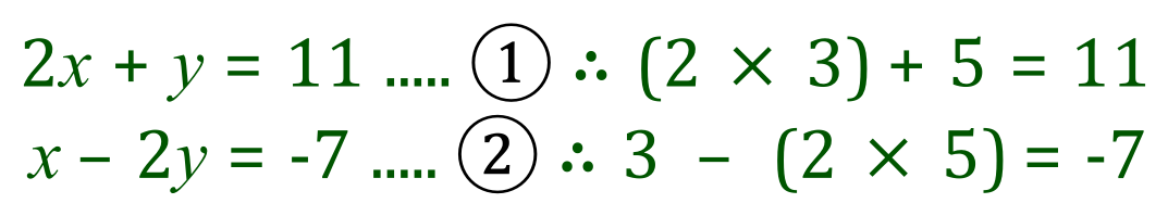
The common point is of course where the lines intersect. You should be able to see that the values of 'x' = 3 and 'y' equals 5 are the values we have been looking for. Substitute these into either of the equations and you will see that they do in fact satisfy both.
>> Questions <<